Melbourne

A groundwater balance for Melbourne region comprises many parts. Groundwater may enter the region via seepage, regional flow and other processes. Groundwater may similarly leave the region via evapotranspiration, lateral flow and other processes.

Each aspect of groundwater movement is calculated and summed to ascertain the change in the volume of groundwater in storage. This value includes all of the inflows and all of the outflows to and from the region.

Change in storage for Melbourne region 2009–10, water table aquifer, is 46,1230 ML.

The change in groundwater storage is estimated for the water table aquifer within the clipped sedimentary area. The groundwater levels were estimated using all bores within the account region. This assumed that all hydrogeological layers are hydraulically inter-connected.

Data source

Victorian Department of Sustainability and Environment: bore locations and groundwater levels data within Port Phillip and Western Port catchment management authorities; aquifer specific yield values from the Port Phillip and Western Port ecoMarkets groundwater model.

Data provider

Victorian Department of Sustainability and Environment and Bureau of Meteorology.

Method

Change in extractable storage was estimated using a simple geographic information system (GIS) approach based on measured groundwater levels and aquifer properties. Firstly, groundwater levels at the start (1 July 2009) and the end (30 June 2010) of the financial year were estimated by interpolating from measurements between March 2009 to October 2009 and March 2010 to October 2010 respectively.

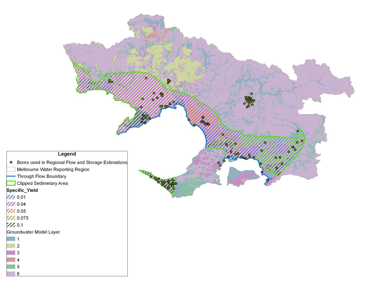
The estimated groundwater levels on a particular date were then spatially interpolated to grids using the ArcGIS Topo-to-Raster tool. The interpolated groundwater level surfaces at the start and the end of financial year were then used to calculate the volume between them within the sedimentary area, shown in the Figure below. Finally, this volume was multiplied by appropriate specific yield values to convert to a change in groundwater storage.

Uncertainty

Uncertainty is ungraded.

The uncertainty in the field-measured data (example: groundwater levels, specific yield) was not specified and hence the impacts of such uncertainty on the change in storage is not estimated.

The change in storage estimations were based on interpolated groundwater level grids produced using the ArcGIS Topo-to-Raster tool. Use of other interpolation methods may impact the values of the groundwater level grids and hence the estimated values for change in groundwater storage.

Approximation, assumptions, caveats/limitation

• The groundwater levels were estimated by assuming that all the hydrogeological layers (excluding basement) within the Port Phillip and Western Port groundwater model region are hydraulically interconnected. This assumption facilitates the interpolation of a groundwater potential surface from groundwater level measurements as these measurements were limited in number. Groundwater levels are also assumed equal to 0 metres Australian Height Datum (mAHD) at the coastline. These assumptions were used to generate groundwater level surfaces across the sedimentary area at the beginning and end of the reporting period.
• Change in groundwater storage was not calculated for confined aquifers. The annual change in storage was considered to be negligible for confined aquifers due to their very low storativity, which is much lower than the specific yield of unconfined aquifers (Freeze and Cherry 1979; Johnson 1967). Upon lowering of water levels in such aquifers, they remain fully saturated so that no dewatering occurs. The water diverted is volumetrically equivalent to the volumetric expansion of the water and contraction of the pore space.
• Annual change in storage in fractured bedrock was considered negligible as the fractures are the only water-holding structures and these systems have a low specific yield. Furthermore, groundwater extraction in fractured rock areas is limited in volume.
• The spatially varying specific yield values considered in the Port Phillip and Western Port ecoMarkets groundwater model (GHD 2010) were used in these estimations.
  
  

Groundwater inflow from outside entity

Data source

Victorian Department of Sustainability and Environment: bore locations and groundwater levels data within Port Phillip and Western Port catchment management authorities; hydraulic conductivity, and aquifer thickness from the Port Phillip and Western Port ecoMarkets groundwater model (GHD 2010).

Data provider

Bureau of Meteorology.

Method

Groundwater flow was calculated using a simple GIS approach based on Darcy’s Law. Groundwater levels were interpolated for each season using the ArcGIS Topo-to-Raster tool from reduced groundwater levels measured at monitoring bores. Seasonal groundwater flow grids were derived from groundwater level grids, aquifer thickness and hydraulic conductivity using a modification of the ArcGIS Darcy Velocity tool. Groundwater flow across selected flow boundaries (figure below) was then calculated using a simple GIS analysis and seasonal values were aggregated to the financial year.

Uncertainty

Uncertainty is ungraded.

The uncertainty in the field measured data (example: groundwater levels, hydraulic conductivity) was not specified and unknown and hence the impacts of such uncertainty on the groundwater flow is not estimated.

The regional flow estimations were based on interpolated groundwater level grids produced using ArcGIS Topo-to-Raster tool. Use of different interpolation methods may impact the values of the groundwater level grids and hence the estimated regional flow.

Groundwater flow was estimated for a simplified boundary constructed from a series of line segments. Groundwater flow across this boundary was calculated using the method described above. The uncertainty surrounding this simplification was not analysed.

Approximations, assumptions, caveats/limitations

• Groundwater levels were estimated by assuming that all the hydrogeological layers within the Port Phillip and Western Port groundwater model region are hydraulically interconnected. This assumption facilitated the interpolation of a groundwater potential surface from groundwater level measurements as these measurements were limited in number. Groundwater levels were also assumed equal to 0 mAHD at the coast line. These assumptions were used to generate seasonal groundwater level surfaces across the sedimentary area.
• Bore locations and the through flow boundaries considered in the estimations are indicated in the figure below. Flow across the remaining boundaries was assumed negligible on an annual basis either because aquifer properties like hydraulic conductivity limit flow (e.g. fractured rock basement), groundwater flow was approximately parallel to the boundary, or limitations of the method used in this estimation did not allow its application (e.g. Nepean Peninsula).

Groundwater recharge

Data sources

Bureau of Meteorology, National Climate Centre (NCC): raster spatial data; version 3, annual rainfall grids; daily maximum temperature grids; daily minimum temperature grids; daily satellite observed solar radiation grids; daily vapour pressure deficit grids; Australian Soil Resources Information System (ASRIS): soil information; Bureau of Rural Sciences Water 2010: land use mapping; Victorian Department of Sustainability and Environment: bore locations and groundwater levels data within Port Phillip and Western Port catchment management authorities.

Data provider

Bureau of Meteorology.

Method

Groundwater recharge and discharge was estimated using the Water Atmosphere Vegetation Energy and Solutes (WAVES) model (Zhang & Dawes 1998; Dawes et al. 1998). WAVES is a one dimensional soil-vegetation-atmosphere-transfer model that integrates water, carbon, and energy balances with a consistent level of process detail. The input data sets required for WAVES include climate, depth to water table, soil and vegetation data. The clipped sedimentary area (Figure above) was selected for the estimation of net recharge. The climate data used at selected points include rainfall, rainfall duration, maximum and minimum temperatures, vapour pressure deficit, and solar radiation. The relevant vegetation parameters required for modelling were selected from the WAVES user manual (Dawes et al. 1998). WAVES uses the soil hydraulic model of Broadbridge and White (1998) with saturated hydraulic conductivity, saturated moisture content, residual moisture content, inverse capillary length scale and an empirical constant as input parameters calculated from soil properties accessed in the ASRIS database (Johnston et al. 2003).

The WAVES model has been used by the CSIRO in its sustainable yields projects (Crosbie et al. 2008) and the Bureau built on this methodology. WAVES was run for all combinations of soil, vegetation, and depth to water table at each climate point. A groundwater recharge value was estimated for each 5 km x 5 km pixel across the region using:

• annual rainfall
• dominant soil and vegetation
• depth to water table.
  

The net recharge within the selected region was estimated based on spatial interpolation of recharge estimates between values at nearby climate points.

Uncertainty

Ungraded.

The uncertainty in the input parameters and the corresponding impacts on the modelled recharge values have not been studied.

The uncertainty of the estimated recharge resulting from different recharge interpolation methods is not estimated.

Approximation, assumptions, caveats/limitations

• Assumptions made in developing the WAVES model as described in Dawes et al. (1998) are all applicable to the recharge estimations carried out for the Melbourne region.
• Bureau of Rural Sciences’ land use map of Melbourne region was reclassified to three vegetation classes that include annuals, perennials and trees. The major vegetation classes modelled are C3 annual pasture, C3 perennial pasture and eucalypt trees with a grass understorey.
• Net recharge was estimated within the clipped sedimentary area (Figure above) considering effects of shallow water table.