Murray–Darling Basin

The Contextual statement of the National Water Account 2010 (the 2010 Account) explains that the many groundwater systems in the Murray–Darling Basin (MDB) region are categorised in three broad types (see Figure 1): 

• alluvial sedimentary systems (Quaternary/Tertiary)
  
• fractured basement rock systems (Paleozoic) 
  
• sediments of the Great Artesian Basin (Cretaceous/Jurassic).

The most significant alluvial sedimentary systems have been included in the groundwater management units (GMUs) on which a water balance is explicitly calculated for the 2010 Account (see Figure 1).

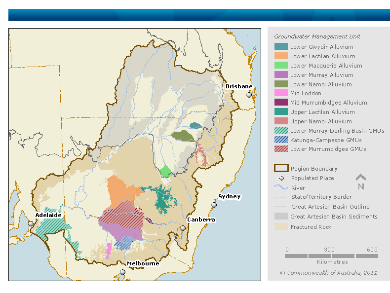
Figure 1. Categories of groundwater systems in the MDB region (Source for boundaries of the region and groundwater management units: Australian Government Department of Sustainability, Environment, Water, Population and Communities, and Murray–Darling Basin Authority)

The annual groundwater balance was conceptualised and calculated in different ways according to the category of groundwater system.

Fractured basement rock aquifers

The fractured rock aquifers shown in Figure 1 are Paleozoic and Precambrian fractured rock geological layers that represent the outcropping hydrogeological basement rock. A notable exception is the Queensland fractured basalts present along the margin of the northeast MDB region). They are predominantly ‘local’ groundwater flow systems with low specific yield (i. e. low groundwater storage capacity) and low hydraulic conductivity. Local groundwater flow systems have groundwater flow paths that are often ≤5 km long, with short response and recession times (in this case, <4 months). Typically, groundwater recharge on a hill slope will discharge at the base of the slope into a small stream a short distance away. At depth, the aquifer hydraulic conductivities are low; therefore, regional groundwater flow is insignificant (i. e. for flow distances ≥100 km). Thus the annual net water flow out of a fractured rock region consists almost entirely of evapotranspiration and streamflow fluxes.

From the perspective of an annual regional water balance calculation, the annual change in stored groundwater volume will usually be insignificant relative to the volume of streamflow or the volume of groundwater discharge to streams. Therefore, the annual water balance calculations in these groundwater systems were simplified by assuming:

• there was no significant annual change in groundwater storage
  
• deep drainage of the rock and soil layers at the land surface occurs as streamflow.

Great Artesian Basin aquifers

The Great Artesian Basin (GAB) has confined aquifer systems at a depth that hold a large volume of water and provide pathways for lateral water movement. Near the land surface there is a thick and largely impermeable confining layer (shale) that separates the soil profile from the GAB aquifers (lying below the GAB outline in Figure 1). Typically, the land surface is very flat and the annual rainfall is low (≤300 mm/yr). Thus the incoming rainfall will largely be lost as evapotranspiration throughout the months following an event. When a wet event occurs (usually once every 5 or 6 years) significant volumes of run-off may be generated (often under flood conditions).

As per the definition of the MDB region (Physical Information of the Contextual statement), groundwater that forms part of the GAB is excluded from the water accounting reports.

Sedimentary/alluvial systems

In contrast with the above two groundwater system types, the alluvial sedimentary aquifers have a high water storage capacity. Their hydraulic conductivity is high enough to allow significant regional groundwater flows. These are the systems for which a calculation of groundwater balance is required to complete an annual regional water balance.

The Contextual statement (Physical Information) explains that, for the purpose of the 2010 Account, the groundwater balance calculation focuses on priority GMUs where groundwater allocations and groundwater extractions are large – typically more than 30 GL per year (see Figure 1). It is estimated that more than 95% of the total allocated groundwater in the MDB region occurs in these GMUs. It should be noted that in much of the remaining areas of the MDB region, the groundwater salinity is high and groundwater is mostly not suitable for irrigation. These remaining areas lie further down the groundwater flow path from the prioritised GMUs.

For most prioritised GMUs, the Bureau of Meteorology applied data-based methods to estimate the following

groundwater flows:

• the groundwater regional flow into and out of the MDB region (Line items 15.1.1 and 16.1.1)
  
• the groundwater flow across the boundary at the coast, both into and out of the MDB region (Line items 15.1.2 and 16.1.2)
  
• the groundwater recharge (Line item 15.2.1) from and discharge to the landscape (Line item 16.3.1)
  
• the changes in groundwater storage.

These methods are described in the specific water accounting statement notes of each line item.

For several prioritised GMUs in New South Wales, the groundwater balance flows were estimated from the outputs of numerical groundwater models run by the NSW Office of Water. These GMUs are Lower Lachlan, Lower Murrumbidgee, mid Murrumbidgee (two models), Lower Namoi, Upper Namoi and Lower Macquarie (see Figure 1).

Besides the line items estimated using data-based methods, the numerical groundwater models outputs also quantified the following line items:

• groundwater recharge from connected surface water (Line item 15. 2. 1) and groundwater discharge to connected surface water (Line item 16. 3. 2)
  
• interbasin inflow into the MDB region from the GAB (in the Lower Namoi GMU) is reported under Line item 15. 1. 3.

Managed aquifer recharge (Line item 15. 2. 6) was quantified for one GMU only, the Angas Bremer Prescribed Wells Area in South Australia, from data provided by the jurisdiction. To date, the volume of managed aquifer recharge is limited and there are very few sites in the MDB region where it is attempted.

Groundwater extractions were evaluated for the prioritised GMUs using jurisdictional data. See the groundwater extractions line items in the water accounting statement notes for details.

Groundwater non-physical flows include:

• decreases – that is, groundwater allocation announcements (see line items 27.1.1, 27.1.2 and 27.1.3.7 in the Statement of Changes of Water Assets and Water Liabilities)
  
• increases – that is, adjustments and forfeiture of groundwater allocations (see line items 28.1.1, 28.1.2 and 28.1.3.7 in the Statement of Changes of Water Assets and Water Liabilities).

According to clause 71 of the Exposure Draft of the Australian Water Accounting Standards 1 (ED AWAS 1), the total volume of groundwater should not be considered as a water asset, because a significant portion of it is non-extractable due to physical and regulatory limitations.

The extractable portion of the groundwater has been evaluated on the basis of long-term average extraction limits set in the jurisdictional groundwater management plans, where those were specified. See Line item 2.3 Aquifers – other lumped in the water accounting statement notes for more detail on the quantifications methods that were used.

As these limits were set at the commencement of the groundwater management plans, the groundwater asset values at 1 July 2009 and 30 June 2010 are the same.

As shown in the water accounting statement notes for Line item 30.3 Unaccounted-for difference – groundwater store, the changes in groundwater asset (closing balance less opening balance) do not reconcile with changes in groundwater assets (increases less decreases) reported during the 2009–10 year. This is likely to be caused by the incomplete coverage of groundwater balance terms calculated for this account as explained in Line item 30.3.

Besides the water balance omponents described above that were reported in the water accounting statements, changes in the groundwater store volume of the water table aquifers during the 2009-10 year were evaluated using aquifer characterisitics and groundwater level measurements (se 'quantification methods' given below).

These values are not reported in the Statement of Changes in Water Assets and Water Liabilities because they represent only changes in physical water stored in the aquifers and not changes in the groundwater asset as defined above.

Table 1 reports on the groundwater changes evaluated for the various GMUs and compares them to the groundwater assets. Table 1 also indicates what method was used to quantify the change in groundwater storage in each GMU: either the Bureau of Meteorology simple method (Bureau method) or the New South Wales groundwater models (NSW models).

With time, trends in the yearly changes in groundwater storages will provide more useful information about the adequacy of the extraction limits set in the groundwater management plans. For instance, a long-term trend of negative changes in groundwater storage may indicate that groundwater in a GMU may be overallocated.

 – = no data available; Bureau = Bureau of Meteorology; NSW = New South Wales; SA = South Australia; Vic = Victoria

Data source

Bureau of Meteorology method (see list of applicable GMUs in Table 1). Bore locations and groundwater level data:

• South Australia: from the Water Regulations (category 2A) information returns provided by South Australian Department for Water
  
• Victoria: from the Department of Sustainability and Environment (DSE) through a database developed by The University of Melbourne (it is possible that small differences between The University of Melbourne database and the DSE groundwater database occur)
  
• New South Wales: from New South of Office of Water (NOW) – PINNEENA groundwater database (version 3.2).

New South Wales groundwater models (see list of applicable GMUs concerned in Table 1):

• outputs of the New South Wales groundwater models.

Data provider

Bureau of Meteorology.

Method

Bureau of Meteorology method (see list of applicable GMUs concerned in Table 1).

Change in extractable storage was estimated using a simple geographical information system (GIS)-approach based on measured groundwater levels and aquifer properties. Firstly, groundwater levels at the start (1 July 2009) and the end (30 June 2010) of the reporting period were interpolated from measurements between March 2009 and October 2009, and March 2010 and October 2010, respectively. The groundwater levels at bore points at 1 July 2009 and 30 June 2010 were then interpolated into grids using the GIS. The groundwater level surfaces are calculated for the water table aquifer only.

The average difference in groundwater level between the two surfaces is calculated for all areas within 20 km of one or more bores. This reduces extrapolation of groundwater levels to areas where there are bores nearby. The average difference in level between the end of year and beginning of year is multiplied by a specific yield value of the water table aquifer, and also the area for which the average difference is calculated. The result is the estimate of volumetric change in storage in the water table aquifer.

Examination of data in the Upper Lachlan catchment revealed high spatial variability in measured groundwater levels. In order to represent groundwater levels accurately, the average difference in groundwater level was calculated for the area within 5 km of one or more bores only, thus restricting the extrapolation of levels. Only 21 bores were available for this assessment in the Upper Lachlan and an area of approximately 1,000 km² of the Upper Lachlan GMU was used in estimating change in storage. NSW groundwater models (see list of applicable GMUs in Table 1):

• model outputs were used to evaluate the changes in groundwater storage
  
• the change in groundwater storage derived from the groundwater models in New South Wales included all the groundwater model layers (not just the water table aquifer layer).

Uncertainty

Uncertainty is ungraded.

The uncertainty in the field-measured data (e. g. groundwater levels, specific yield) was not specified and hence the impacts of such uncertainty on the change in storage was not estimated.

The change in storage estimations were calculated from the interpolated groundwater level grids produced using ArcGIS Topo-to-Raster tool. Use of other interpolation methods may impact the values of the groundwater level grids and hence the estimated values for change in groundwater storage.

Approximation, assumptions, caveats/limitation

Bureau of Meteorology method (see list of applicable GMUs in Table 1):

• Change in groundwater storage was not calculated for confined aquifers. The annual change in storage is considered to be negligible for confined aquifers due to their very low storage coefficient, which is much lower than the specific yield of unconfined aquifers (Freeze & Cherry 1979; Johnson 1967). As long as confined aquifers remain saturated, changes in piezometric levels (i. e. aquifer pressure) usually cause small changes in water volumes stored in the aquifers; the changes are equivalent to the volumetric expansion/contraction of the water and the pore space.
  
• A constant specific yield value of 0.1 was used for water table aquifers in the estimations as an approximation consistent with some values in the literature.

NSW groundwater models (see list of applicable GMUs concerned in Table 1).

• not available.

The groundwater balance was estimated using the conceptualisation described above for each of the three categories of groundwater systems within the MDB region distinguished for the 2010 Account.

Although there are some areas within the region that are not within these three categories and thus not yet accounted for, it is assumed that these areas are much less significant to an annual water balance of the region. These areas are typically in zones with low rainfall and high groundwater salinity.